First, there are 51 (of 860 total) posts with zero likes and zero tweets. This is important information: these are posts that no one thought worthy of social media attention. Unlike Causal Loop, I want to keep these data in my dataset.
Second, instead of a ratio of likes to tweets (or more precisely, an index based on a modified ratio), I'll estimate separate models for likes and tweets, with comparable specifications. To see the problem with ratios consider the following three posts
Post A: 4 tweets, 2 likes
Post B: 8 tweets, 2 likes
Post C: 400 tweets, 200 likes
A ratio metric treats posts A and C as identical, while separating them from post B. But intuitively we expect a post like C, which generates a lot of social media activity in aggregate, to be different from posts A and B, which don't. (This scale insensitivity is a general characteristic of ratio measures.) This is one of the reasons I prefer disaggregate models. Another reason is that adding Google "+1"s would be trivial to a disaggregate model -- just run the same specifications for another dependent variable -- and complex to a ratio-based index.
To test various hypotheses one can use appropriate tests on the coefficients of the independent variables in the models or simulations to test inferences when the specifications are different (and a Hausman-like test isn't conveniently available). That's what I would do for more serious testing. With identical specifications one can compare the z-values, of course, but that's a little too reductive.
Since the likes and tweets are count variables, all that is necessary is to model the processes generating each as the aggregation of discrete events. For this post I assumed a Poisson process; its limitations are discussed below.
I loaded Causal Loop's data into Stata (yes, I could have done it in R, but since the data is in Stata format and I still own Stata, I minimized effort) and run a series of nested Poisson models: first with only the basic descriptor variables (length, graphics, video, grade level), then adding the indicator variables for the authors, then adding the indicator variables for the topics. The all-variables-included models results (click for bigger):
A few important observations regarding this choice of models:
1. First and foremost, I'm violating the Prime Directive of model-building: I'm unfamiliar with the data. I read the Monkey Cage regularly, so I have an idea of what the posts are, but I didn't explore the data to make sure I understood what each variable meant or what the possible instantiations were. In other words, I acted as a blind data-miner. Never do this! Before building models always make sure you understand what the data mean. My excuse is that I'm not going to take the recommendations seriously and this is a way to pass the morning on Saturday. But even so, if you're one of my students, do what I say, not what I just did.
2. The choice of Poisson process as basis for the count model, convenient as it is, is probably wrong. There's almost surely state dependence in liking and tweeting: if a post is tweeted, then a larger audience (Twitter followers of the person tweeting rather than Monkey Cage readers) gets exposed to it, increasing the probability of other tweets (and also of likes -- generated from the diffusion on Twitter which brings people to the Monkey Cage who then like posts to Facebook). By using Poisson, I'm implicitly assuming a zero-order process and independence between tweets and likes -- which is almost surely not true.
3. I think including the zeros is very important. But my choice of a non-switching model implies that the differences between zero and other number of likes and tweets is only a difference of degree. It is possible, indeed likely, that they are differences of kind or process. To capture this, I'd have to build a switching model, where the determinants of zero likes or tweets were allowed to be separate from the determinants of the number of tweets and likes conditional on their being nonzero.
With all these provisos, here are some possible tongue-in-cheek conclusions from the above models:
Joshua Tucker doesn’t influence tweetability, but his authorship decreases likability; ditto for Andrew Gelman and John Sides. Sorry, guys.
James Fearon writes tweetable but not likable content.
Potpourri is the least tweetable tag and also not likable; International relations is the most tweetable but not likable; Frivolity, on the other hand is highly likable. That says something about Facebook, no?
Newsletters are tweetable but not likable… again Nerds on Tweeter, Airheads on Facebook.
As for Joshua Tucker's hypotheses, I find some support for them, from examining the models, but I wouldn't want to commit to a support or reject before running some more elaborate tests.
Given my violation of the Prime Directive of model building (make sure you understand the data before you start building models), I wouldn't start docking the -- I'm sure -- lavish pay and benefits afforded by the Monkey Cage to its bloggers based on the numbers above.
I've now watched a significant portion of Andrew Ng's Stanford Machine Learning course on iTunes U. I have taken several Machine Learning [classroom] courses, I've read many Machine Learning books and technical papers, I've done research on Machine Learning, and I've also taught Machine Learning. In short, I already know all the material in this course; watching it is mostly entertainment and professional curiosity.
And I still find the lectures harder to follow than a simple textbook.
(That's a lecture format problem, not a Andrew Ng problem.) The supplemental materials help, but they are essentially class notes in PDF format. (There are some problem sets, but no affordances for the general audience to get them graded.)
In lieu of, or to complement, this online course, here are a couple of non-interactive Machine Learning textbooks available online -- legally; posted by their authors:
Yes, an interactive textbook with Matlab (or Octave or R) programming affordances would be better than a non-interactive textbook, especially if the reader received feedback on his/her performance. But I still don't see the point of watching someone talk through the ML points when reading them is much faster. Video is useful when demonstrating software, for example, but a screen capture would work better than a classroom shot for that.
Let me reiterate the golden rule of learning technical material: 1% lecture, 9% study, 90% practice. You still need the textbook (preferably with dynamic content where applicable and programming and testing affordances) and the job of the instructor is crucial (selecting the material, sequencing it, choosing the textbook, designing the assignments, grading the assignments; and someone must write the textbook, of course), but the learning happens when you can WRITE CODE AND INTERPRET RESULTS.
If that's hard on your self-esteem, then tough. Machines don't care.
I've noticed that some smart people I know have different views of the world. Not just social, cultural, political, or aesthetic. They really do see the world through different conceptual lenses: mine are quantitative, theirs are qualitative.
Let's keep in mind that these are smart people who, when prompted to do so, can do basic math. But many of them think about the world in general, and most problems in particular, in a dequantified manner or limit their quantitative thinking in ways that don't match their knowledge of math.
Level 1 - Three different categories for quantities
Many people seem to hold the the three-level view of numbers: all quantities are divided into three bins: zero, one, many. In a previous post I explain why it's important to drill down into these categories: putting numbers in context requires, first of all, that the numbers are actual numbers, not categorical placeholders.
This tripartite view of the world is particularly bad when applied to probabilistic reasoning, because the world then becomes a three-part proposition: 0 (never), 50-50 (uncertain, which is almost always treated as the maximum entropy case), or 1 (always).
Once, at a conference, I was talking to a colleague from a prestigious school who, despite agreeing that a probability of 0.5 is different from a probability of 0.95, proceeded to argue his point based on an unstated 50-50 assumption. Knowing that $0.5 \neq 0.95$ didn't have any impact in his tripartite view of the world of uncertainty.
The problem with having a discussion with someone who thinks in terms of {zero, one, many} is that almost everything worth discussing requires better granularity than that. But the person who thinks thusly doesn't understand that it is even a problem.
Level 2 - Numbers and rudimentary statistics
Once we're past categorical thinking, things become more interesting to quantitatively focused people; this, by the way, is where a lot of muddled reasoning enters the picture. After all, many colleagues at this level of thinking believe that, by going beyond the three-category view of numbers, they are "great quants," which only proves the Dunning-Krueger effect applies.
For illustration we consider the relationship between two variables, $x$ and $y$, say depth of promotional cut (as a percentage of price) and promotional lift (as a percentage increase in unit sales due to promotion). Yep, a business example; could be politics or any social science (or science for that matter), but business is a neutral field.
At the crudest level, understanding the relationship between $x$ and $y$ can be reduced to determining whether that relationship exists at all; usually this is done by determining whether variation in one, $x$, can predict variation in the other, $y$. For example, a company could run a contrast experiment ("A-B test" for those who believe Google invented experiments) by having half their stores run a promotion and half not; the data would then be, say:
Sales in stores without promotion: 200,000 units/store
Sales in stores with promotion: 250,000 units/store
Looks like a relationship, right? An apparent 25-percent lift (without knowing the depth of the price cut I can't comment on whether this is good or bad). But what if the average sales for all stores when there are no promotions on any store is 240,000 units/store? All this promotion apparently did was discourage some customers in the stores without promotions (the customers know about the promotion in other stores because you cannot stop information for diffusing over social media, for example) and incentivize a few of the discouraged to look for the stores running the promotion.
(A lot of anecdotes used to support public policy make the sort of mistake I just illustrated. There are plenty of other mistakes, too.)
To go beyond the simple observation of numbers and to use statistical tests, we need to have some formulation of the relationship, for example a linear one such as:
$\qquad y = \beta \, x + \epsilon$.
This formulation includes a term $\epsilon$ (called stochastic disturbance) which is the modeler's admission that we don't know everything we'd like to. (All tests have an underlying structure, even non-parametric tests; when people say that there's no structure what they are really saying is that they don't understand how the test works.)
Given some pairs of observations $\{(x_1,y_1), (x_2,y_2),\ldots\}$ , the relationship can be tested by estimating the parameter $\beta$ and determining whether the estimate $\hat \beta$ is significantly different from zero. If it's not, that means that the value of $y$ is statistically independent of $x$ (to the level of the test) and there is no relationship between them -- as far as statistical significance is concerned.
There's a lot to argue about significance testing, some of which I put in this video:
Once we get past simple tables and possibly the prepackaged statistical tests that can be done on these tables -- almost like an incantation with statistical software taking the place of the magical forces--, few people remain who want to discuss details. But even within that small set, there are many different sub-levels of thinking.
Level 3 - Thinking in models and functions
Let's go back to the linear formulation in $y = \beta \, x + \epsilon$. What this means is that lift $y$ increases with price cut $x$ in a proportional way, independent of the magnitudes of each.
Ok, so what? ask a lot of people whose level of numerical reasoning is being stretched. The "what" is that the effect of a change of price cut from 4 to 5 percent is assumed to be equal to that effect of the change from 45 to 46 percent. And this assumption is probably not true (actually, empirically we have evidence that this is not true).
Many people are able to repeat the rationale in the previous paragraph, but don't grok the implications.
The questions of where we go from this simple model are complicated. Let us ignore questions of causality for now, and focus on how different people want perceive the importance of details in the relationship between $x$ and $y$.
Increasing vs decreasing. Almost everyone who gets to this level of thinking cares about the direction of the effect. At this stage, however, many people forget that functions may be monotonic (increasing or decreasing) over an interval while outside that interval they may become non-monotonic (for example, increasing until a given point and then decreasing).
Convex versus concave. Even when the function is monotonic over the interesting domain, there's a big difference between linear, convex, and concave functions. Some disagreements with very smart people turned out to be over different assumptions regarding this second derivative: implicitly many people act as if the world is either linear or concave (assuming that the effect of adding 1 to 10 is bigger than the effect of adding 1 to 1000). As I pointed out in this post about network topologies and this post about models, combinatorics has a way of creating convexities. There's also a lot of s-shaped relationships in the world, but we'll leave those alone for now.
Functional form. As I illustrated in my post on long tails, two decreasing convex functions (the probability mass functions of the Poisson and Zipf distributions) can have very important differences. Empirical researchers are likely to care more about this than theoretical modelers, but once we reach the stage where we are discussing in these terms (and the group of people who can follow and participate in this discussion) arguments tend to be solved by mathematical inference or model calibration. In other words, leaving personal issues and inconvenient implications aside.
(Needless to say -- but I'll write it anyway -- this is the level of discussion I'd like to have when consequences are important. Alas, it's not very common; certainly not in the political or social sciences arena. In business and economics it's becoming more common and in STEM it's a foundation.)
Elaboration is still possible. I'll illustrate by noting that underlying assumptions (that I never made explicit, mind you) can come back to bite us in the gluteus maximus.
(Non-trivial statistics geekdom follows; skip till after the next picture to avoid some technical points about model building.)
Let's assume that we collect and store the data disaggregate by customer, so that $y_i$ is the quantity (not lift) bought by customer $i$; after all, we can always make aggregate data from disaggregate data but seldom can do the opposite. How would we analyze this data?
First observation: expenditures per customer are greater than zero, always. But our model might predict, for some values of $\epsilon$ a negative prediction for $y_i$ times price (which is a positive number). So our model needs to be tweaked to take into account the hard bound at zero.
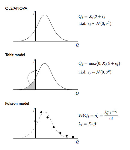
If ours were retail stores, where the data collected by the PoS scanners is only available for customers who buy something (in other words, we don't observe $y$ when $y=0$), we would have to use a technique called a censored regression; if we observe the zeros (like on a online retail site), then a model called Tobit will account for the pooling of the probability mass at zero.
Second observation: the number of units bought by any given customer is an integer; we keep treating it as a continuous quantity. Typically regression models and their variants like censored regression and Tobit assume that the stochastic disturbances are Normal variables. That would lead to possible $y_i = 1.35$, which is nonsensical in our new data: $y_i \in \{0,1,2,3,\ldots\}$.
Counting models, like a Poisson regression (which has its own assumptions) take the discreteness into account and correct the problems introduced by the continuity assumption. In olden days (when? the 50s?) these were hard models to estimate but now they are commonly included in statistical packages so there is no reason not to use them.
For illustration, here's what these models look like:
Conclusion - why is it so hard to explain these things?
Thinking quantitatively is like a super-power: where others know of phenomena, we know how much of a phenomenon.*
The problem is that this is not like a amplifier super-power, like telescopic vision is to vision, but rather an orthogonal super-power, like the ability to create multiple instances of oneself. It's hard to explain to people without the super-power (people who don't think in numbers, even though they're smart) and it's hard to understand their point of view.
Contrary to the tagline of the television show Numb3rs, not everyone thinks in numbers.
That's a pity.
-- -- -- --
* A tip of the hat to Dilbert creator Scott Adams, via Ilkka Kokkarinen's blog for pointing this out in a post which is now the opening chapter of his book.